Irrigation scheduling addresses two critical questions: when to irrigate and how much water to apply. Providing the optimal amount of water at the right time enhances water use efficiency, leading to improved crop production, while minimizing water losses and ensuring sustainable water management. This article compares two widely used soil water balance-based irrigation scheduling methods—Checkbook and FAO-56—by evaluating their principles, advantages, and limitations, with a focus on how each method tracks and manages soil moisture. To illustrate their differences, we present example calculations demonstrating how each method estimates irrigation timing and amount. The Checkbook Method is widely adopted for its simplicity, while FAO-56 offers greater accuracy and is better suited for long-term irrigation planning. By presenting both approaches, followed by a practical “Which Method is Right for Me?” decision guide, this article serves as a valuable resource for farmers, extension specialists, and irrigation managers, helping them choose a method that aligns with their needs and management goals.
Introduction
Irrigation scheduling helps farmers decide when to irrigate and how much water to apply so that soil moisture stays at levels that support healthy plant growth. Too little water can cause water stress, which occurs when a plant’s water requirement exceeds water uptake from the soil, creating a water deficit in the crop root zone and reducing yields. Too much irrigation, on the other hand, can lead to waterlogging, where excess water fills the soil and prevents roots from getting enough oxygen, increasing disease risks in crops that are sensitive to low levels of soil oxygen, such as tobacco, maize, and potatoes.1,2 Over-irrigation also wastes money on water, fertilizer, and labor, and can degrade groundwater quality through the leaching of nitrates, salts, and pesticides.1,3
Efficient irrigation scheduling can significantly enhance water-use efficiency while reducing unnecessary losses.4 Studies conducted in Nebraska have shown that proper irrigation scheduling can save up to 35% of water and energy costs.5 Scheduling also becomes critical when water resources are limited, allowing irrigation managers to strategically apply water at growth stages where crops can tolerate moderate stress without significant yield reductions.
Several irrigation scheduling tools are available, from soil moisture sensors (e.g., soil probes) to soil water balance (SWB) methods. Soil moisture sensors provide real-time data, enabling farmers to decide whether irrigation is needed. SWB methods, on the other hand, track soil moisture by recording all water inputs (e.g., irrigation, rainfall) and outputs (e.g., crop water use). These methods estimate soil moisture status without requiring expensive sensors, making them a cost-effective alternative. Two widely used SWB methods are:
- The Checkbook Method – A manual, spreadsheet-based approach that estimates soil moisture changes using crop water use (ETc), rainfall, and irrigation inputs. It simplifies the soil water balance by relying on fixed assumptions for crop water use.
- The FAO-56 Method – A standardized approach that separately accounts for transpiration from vegetation and evaporation from soil. It provides a more comprehensive soil water balance by dynamically tracking soil moisture while considering crop growth stages, changes in root zone depth, and crop water stress.
While the FAO-56 Method relies on software programs like CROPWAT6 or the FAO ETo calculator,7 the Checkbook Method can be done by hand with pen and paper, or with a simple spreadsheet. The choice between Checkbook and FAO-56 methods has implications not only for farmers and irrigation managers but also for extension specialists, extension agents, and policymakers involved in sustainable irrigation planning. While farmers prefer the Checkbook Method for its simplicity, its lack of precision can lead to errors in scheduling and potentially impact crop yields. In contrast, FAO-56 provides a more systematic approach, making it a valuable tool for effective irrigation scheduling and water management decisions in large-scale agricultural operations. This publication compares these two SWB-based scheduling methods and provides guidance on selecting the most appropriate approach based on management needs and the desired level of accuracy.
Definition of Key Terms
| Term | Definition |
| (Crop) Water Demand | Amount of water a crop needs for optimal growth under ideal conditions, assuming no water stress. |
| (Crop) Water Use / Crop Evapotranspiration (ETc) | Amount of water lost through evaporation from the soil surface and transpiration from plant leaves, representing the total amount of water used by the crop. |
| (Crop) Water Stress | Condition when soil moisture is insufficient to meet crop water demand, causing reduced growth and water use. |
| Runoff | Portion of rainfall and irrigation water that flows over the soil surface instead of infiltrating into the soil. |
| Deep Percolation | Downward movement of water beyond the root zone when soil water exceeds its storage capacity and is no longer available to plants. |
| Capillary Rise | Upward movement of water from groundwater into the root zone through small pores in the soil, similar to water climbing up a paper towel dipped in a glass of water. |
| Field Capacity | Amount of water remaining in soil after excess water has drained away, similar to a sponge that is fully soaked and cannot hold any more water. |
| Wilting Point | Soil water content below which plants cannot extract water, causing permanent wilting. |
| Total Available Water (TAW) | Total water available to plants within the root zone. |
| Readily Available Water (RAW) | Portion of TAW that can be used by plants without causing water stress. |
| Soil Water Depletion Fraction (p) | Ratio of RAW to TAW that defines when a crop begins experiencing water stress. |
| Management Allowed Depletion (MAD) | Fraction of TAW that can be depleted before irrigation is applied. |
| Reference Evapotranspiration (ETo) | Evapotranspiration rate from a reference surface of dense, actively growing grass, about 0.12 m tall and not short of soil water. |
| (Single) Crop Coefficient (Kc) | Factor used to convert ETo into ETc, reflecting crop type and growth stage. |
| Basal Crop Coefficient (Kcb) | Portion of the crop coefficient that represents water loss through plant transpiration only. |
| Evaporation Coefficient (Ke) | Portion of the crop coefficient that represents water loss due to evaporation from the soil surface. |
| (Water) Stress Coefficient (Ks) | Factor that reduces crop water use when soil moisture falls below the RAW level. |
Checkbook Method
The Checkbook Method of irrigation scheduling allows farmers to monitor daily soil water balance by tracking crop water use, rainfall, soil moisture deficit, and irrigation in terms of inches or millimeters (mm) of water.3 In simple terms, this method functions like managing a checking account: water added to the soil through irrigation or rainfall acts as a deposit, while water lost through crop water use, also known as crop evapotranspiration (ETc), functions as a withdrawal.8,9 Just as maintaining a balanced checkbook prevents overspending, tracking soil moisture helps to ensure that plants receive the right amount of water at the right time.
Many farmers prefer this method due to its simplicity—it requires tracking only a few key components and allows for manual recording of daily changes to calculate soil water deficits using structured, easy-to-follow steps. However, it has several limitations. It does not account for water losses due to deep percolation and runoff, and relies on a simplified representation of soil water balance processes. Additionally, it does not consider root depth variations. These limitations make the Checkbook Method less precise, leading to suboptimal irrigation scheduling. Therefore, this method is generally more suitable for simpler applications where ease of use is prioritized over precision.
There are various irrigation scheduling tools available that utilize the Checkbook Method. Printable soil water balance sheets that can be manually filled out and used in the field by farmers are available in Scherer8 and Melvin9 and can also be downloaded from the MSU’s Soil Water Balance Sheet.10 A spreadsheet-based version, MSU Irrigation Scheduler, can be downloaded from MSU’s website.10 Additionally, Irris Scheduler, developed by Purdue University’s Department of Agronomy, is a software tool designed for irrigation scheduling and is available at Purdue Irrigation Scheduler.10
To successfully implement this method, three key components must be determined: (1) available water capacity (AWC) and management allowed depletion (MAD), (2) crop water use, and (3) rainfall and irrigation amounts. By monitoring these values, farmers can easily assess soil moisture levels daily and determine when irrigation is necessary.
Available Water Capacity and Management Allowed Depletion
Soil acts as a reservoir, holding water from rainfall and irrigation. However, once it reaches field capacity, any excess water either percolates deeper into the ground or runs off into nearby water bodies. This means over-irrigation beyond field capacity wastes both water and energy and can cause environmental degradation. While soil moisture is available to plants, not all of it can be extracted. As plants use soil moisture, the water content decreases until it reaches the wilting point—when water is so tightly bound to soil particles that plant roots can no longer absorb it. Beyond this point, crops experience severe water stress and may not survive. The difference between field capacity and wilting point determines the AWC, which varies based on soil type. AWC, thus refers to the total amount of water stored in the soil that is accessible for plant uptake. Farmers can find AWC values for their specific soil type using the NRCS Soil Survey.11
While AWC indicates the amount of water the soil can store for plants, the total available water (TAW) refers to how much of that water is actually held within the crop’s rooting depth. To prevent excessive crop stress, however, irrigation should be applied before the soil moisture reaches the wilting point. Growers and irrigation managers usually allow a certain percentage of available soil water to be depleted before irrigation is necessary—this is called the MAD. They typically set MAD at 50% of TAW, although it may range from 40% to 60% depending on crop type, to ensure irrigation is scheduled before moisture levels become critically low. When planning irrigation schedules, they typically select a specific MAD value for the entire growing period.
Crop Water Use
Crop water use, also known as crop evapotranspiration (ETc) is a crucial indicator of a crop’s water demand throughout its growth cycle. Understanding ETc helps farmers and irrigation managers optimize irrigation schedules to ensure crops receive the right amount of water at the right time. In the Checkbook Method, several approaches are used to estimate ETc, with the choice depending on data availability and accuracy requirements.
One approach is to use local crop water use curves, which estimate a crop’s water usage at various growth stages. Because crop water use is strongly influenced by local climate, the magnitude of these curves can vary considerably from one region to another. For this reason, irrigation scheduling is generally more accurate when locally developed crop water use curves are available. Figure 1, adapted from Evans et al.,12 shows a typical corn water use curve across its development. The curve indicates that corn uses water nearly three times more during the pollination period (65-75 days after planting, ~0.25 inch per day) compared to the knee-high stage (35-40 days after planting, ~0.08 inch per day). Similarly, crop water use tables provide empirically derived ETc estimates for specific crops using growth stage and maximum temperature categories. Interested readers can refer to Tables 6 to 14 of Scherer et al.,8 which provide average daily water use for irrigated crops in North Dakota across different growth periods. While these methods are simple and easy to implement, they vary based on location, as local weather conditions influence crop water demand. Another method for estimating ETc is using pan evaporation (Ep), which involves measuring the evaporation of water from a standardized pan. This value can be obtained from weather stations and is multiplied by the pan coefficient (Kp) to determine ETc. Although this method can be useful, it is less commonly applied because weather stations that measure Ep are often located far from the farm, making these values unreliable for localized irrigation scheduling.
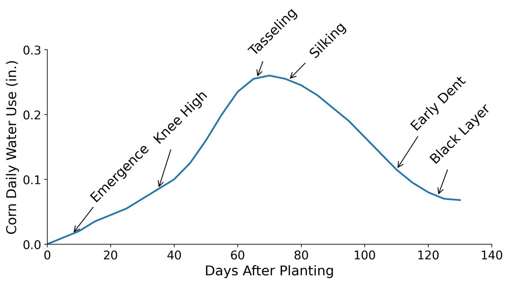
Figure 1. Corn daily water use curve at different growth stages (adapted from Evans et al.12).
The most widely used method for estimating ETc is based on ETo. ETo values are provided by the National Weather Service (NWS), which even offers a 7-day forecast of ETo across the U.S. through its Graphical Forecasts website.13 ETc is then calculated by multiplying ETo with a crop coefficient (Kc). This approach, known as the single crop coefficient method in FAO-56, has been integrated into the Checkbook Method’s soil water balance sheets, making it widely used by farmers and irrigation managers. As shown in Figure 2, Kc values vary with the growth stage of a crop. Early in the season, when the plant canopy is small, crop water use (ETc) is low, and Kc values are correspondingly small (Kc ini). As the plant develops, ETc increases and reaches its maximum when the canopy is fully developed (Kc mid). Toward the end of the season, as the crop reaches physiological maturity, water use declines again (Kc end). These seasonal patterns are reflected in Table 1, which provides Kc values together with approximate stage lengths for major agronomic crops at different growth stages, partially adapted from Allen et al.14 Using ETo for ETc calculations is advantageous because it accounts for local weather conditions, making the estimates more accurate. For example, even if crop water curves suggest high water use during peak growth, actual water demand may be lower on cool, humid days. This approach allows farmers to adjust irrigation schedules based on real-time weather forecasts, improving water use efficiency and helping to prevent over-irrigation.
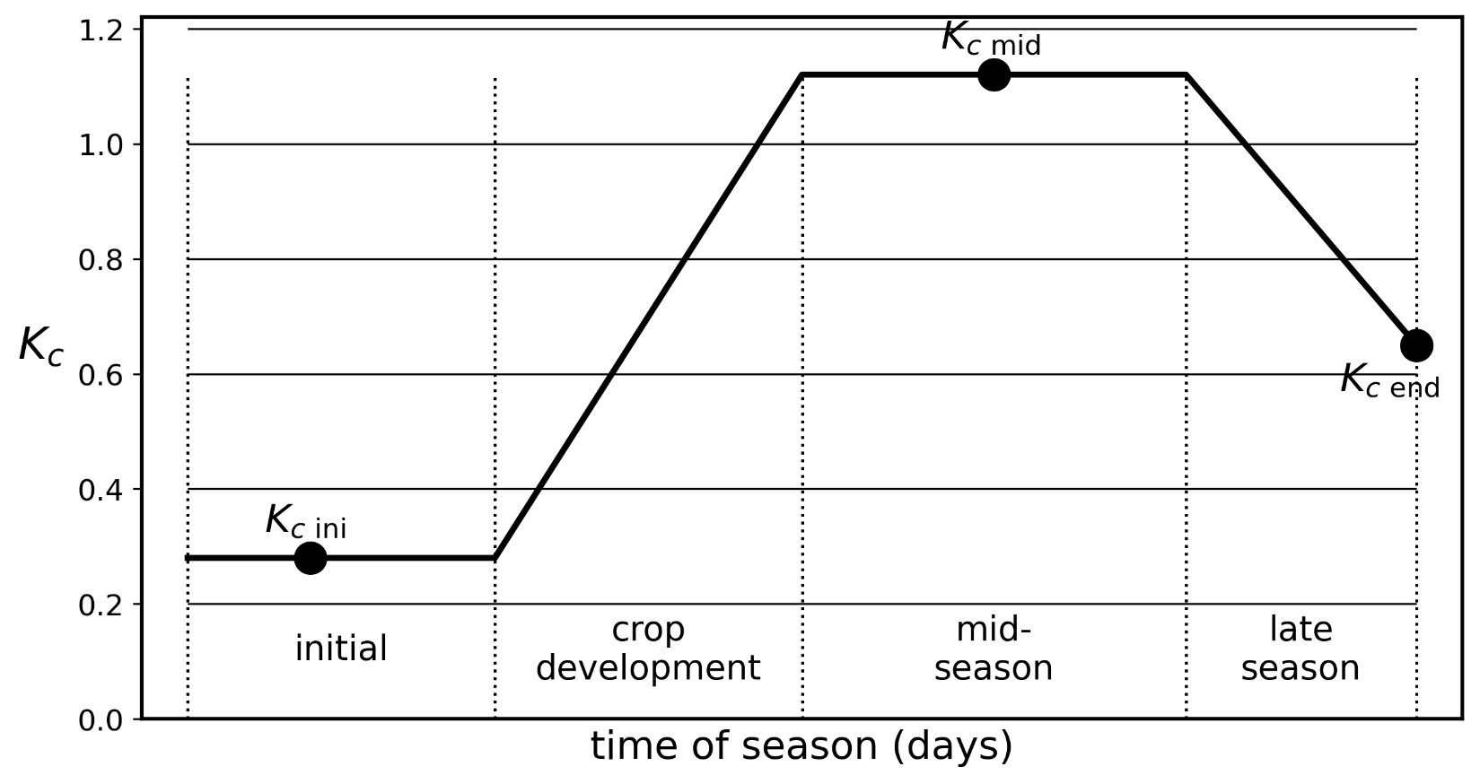
Figure 2. Schematic crop coefficient (Kc) curve showing how Kc changes across the initial, crop development, mid-season, and late-season growth stages (adapted from Allen et al.14)
Table 1. Crop Coefficients (Kc) and Approximate Crop Development Stage Lengths for Major Agronomic Crops (partially adapted from Allen et al.14)
| Crop | Kc ini | Kc mid | Kc end | Ini. (d) | Dev. (d) | Mid (d) | Late (d) |
| Corn | 0.3 | 1.15 | 1.05 | 20-30 | 20-40 | 25-70 | 10 |
| Soybeans | 0.4 | 1.15 | 0.5-1.0 | 15-20 | 15-35 | 40-75 | 15-30 |
| Cotton | 0.35 | 1.15-1.2 | 0.5-0.7 | 30-45 | 50-90 | 45-60 | 45-55 |
| Wheat | 0.3 | 1.15 | 0.25-0.4 | 15-40 | 25-60 | 40-65 | 20-40 |
| Groundnut | 0.4 | 1.15 | 0.6 | 25-35 | 35-45 | 35-45 | 25-35 |
| Grapes | 0.8 | 1.15 | 0.85 | 20-30 | 40-60 | 40-120 | 20-80 |
| Sweet Potatoes | 0.5 | 1.15 | 0.65 | 15-20 | 30 | 50-60 | 30-40 |
| Broccoli | 0.7 | 1.05 | 0.95 | 35 | 45 | 40 | 15 |
| Asparagus | 0.5 | 0.95 | 0.3 | 50-90 | 30 | 100-200 | 45-50 |
Note: Here, Kc ini refers to the early season, Kc mid to peak growth, and Kc end to the end season Kc values, while Ini., Dev., Mid, and Late indicate the approximate duration, in days (d), of the initial, crop development, mid-season, and late-season stages, respectively. Stage lengths are general ranges and may vary with region, climate, and local growing conditions.
Rainfall and Irrigation Amount
In addition to crop ETc, the Checkbook Method also requires recording the amount of rainfall and irrigation applied to the field. Rainfall data can be accessed from nearby weather stations using National Oceanic and Atmospheric Administration’s (NOAA) Climate Data Online Search tool.15 If weather station data is unavailable, farmers can install rain gauges in the field to measure rainfall directly. Similarly, irrigation amounts should be recorded to ensure accurate tracking of soil moisture levels.
Soil Water Balance Calculation
Once AWC of the soil, ETc, rainfall, and irrigation data are known, farmers can maintain a daily soil water balance, updating moisture levels using the following equation:
WBi = WBi-1 + Pi + Ii – ETci (1)
where, WBi and WBi-1 represent the water balance at the end of the current (i) and previous day (i-1). Pi is the daily rainfall, Ii is the daily net irrigation depth, and ETci is the daily evapotranspiration for the current day, with all terms measured in water depth units (in). This equation allows for daily updates, helping farmers to plan irrigation applications more effectively.
Table 2 provides an example of soil water balance tracking using the Checkbook Method over two successive weeks, partially referenced from Example 38 of Allen et al.14. A MAD of 50% is considered, meaning irrigation is applied once the soil water deficit approaches this threshold. Both irrigation and rainfall are assumed to occur early in the day.
Table 2. Example of a Soil Water Balance Tracking Table Using Checkbook Method for Irrigation Scheduling
| Day | ETo (in) | SWB (in) | P (in) | I (in) | Kc | ETc (in) | EWB (in) | Soil Water deficit (%) |
| 1 | 0.18 | 1.54 | 0 | 1.57 | 0.40 | 0.07 | 1.47 | 5 |
| 2 | 0.20 | 1.47 | 0 | 0 | 0.40 | 0.08 | 1.39 | 10 |
| 3 | 0.15 | 1.39 | 0 | 0 | 0.40 | 0.06 | 1.33 | 14 |
| 4 | 0.17 | 1.33 | 0 | 0 | 0.40 | 0.07 | 1.26 | 18 |
| 5 | 0.19 | 1.26 | 0 | 0 | 0.40 | 0.08 | 1.18 | 23 |
| 6 | 0.11 | 1.42 | 0.24 | 0 | 0.40 | 0.04 | 1.38 | 10 |
| 7 | 0.23 | 1.38 | 0 | 0 | 0.40 | 0.09 | 1.29 | 16 |
| 8 | 0.20 | 1.29 | 0 | 0 | 0.40 | 0.08 | 1.21 | 21 |
| 9 | 0.19 | 1.21 | 0 | 0 | 0.40 | 0.08 | 1.13 | 27 |
| 10 | 0.20 | 1.13 | 0 | 0 | 0.40 | 0.08 | 1.05 | 32 |
| 11 | 0.22 | 1.05 | 0 | 0 | 0.40 | 0.09 | 0.96 | 38 |
| 12 | 0.22 | 0.96 | 0 | 0 | 0.40 | 0.09 | 0.87 | 44 |
| 13 | 0.20 | 0.87 | 0 | 0 | 0.40 | 0.08 | 0.79 | 49 |
| 14 | 0.19 | 1.50 | 0 | 0.71 | 0.40 | 0.08 | 1.42 | 8 |
Note. ETo and ETc represent reference and actual crop evapotranspiration, Kc is the crop coefficient, P and I denote rainfall and irrigation amounts, and SWB and EWB are starting and ending soil water balance, respectively. The highlighted soil water deficit on Day 13 (49%) shows the value is approaching the MAD threshold (50%), and therefore irrigation is applied the following day.
The example assumes:
- Root zone depth (Zr): 11.81 in on Day 1.
- Soil type: Sandy loam with a field capacity (θFC) of 0.23 in³/in³ and a wilting point (θWP) of 0.10 in³/in³.
- TAW: Calculated as:
TAW = (θFC – θWP) × Zr = (0.23-0.10) × 11.81 = 1.54 in
- Reference evapotranspiration (ETo): Given.
- Irrigation (I) and Rainfall (P): 1.57 in irrigation on Day 1 and 0.24 in rainfall at the beginning of Day 6.
- Starting soil water balance (SWB): At the start of Day 1, SWB is assumed to be at the MAD threshold. However, 1.57 in of irrigation is applied early on Day 1. If total input (P + I) exceeds TAW, SWB is limited to TAW. Since TAW is 1.54 in, the SWB for Day 1 is set to 1.54 in. From Day 2 onward, SWB is determined as:
SWBi = EWBi-1 + Pi + Ii (2)
If SWB exceeds TAW, it is capped at TAW.
- Crop coefficient (Kc): Determined from the stage-based Kc values in Table 12 together with the crop development stage lengths in Table 11 of Allen et al.14
- Crop water use (ETc): Calculated as:
ETc = Kc × ETo (3)
- Ending soil water balance (EWB): Computed as:
EWBi = SWBi – ETc (4)
- Soil water deficit (%): Indicates the percentage of soil water depletion relative to TAW. Since MAD is 50%, irrigation is needed when this threshold is approached to prevent crop water stress.
The interpretation of the moisture trend is detailed below:
- Early period (Days 1–5): Soil moisture is adequate due to the initial 1.57 in irrigation, and the water deficit remains low.
- Midway (Days 6–10): A small rainfall event (0.24 in) on Day 6 provides some replenishment, but evapotranspiration gradually reduces soil moisture over the following days.
- Critical period (Days 11–13): By Day 13, the water deficit reaches 49%, nearing the 50% MAD threshold, indicating an urgent need for irrigation.
- Irrigation event (Day 14): An 0.71 in irrigation is applied, ensuring soil moisture is replenished without exceeding TAW, thereby preventing crop water stress.
FAO-56 Method
The FAO-56 Method follows a water balance approach similar to the Checkbook Method but incorporates more detailed calculations to account for crop water use, soil water availability, and environmental factors. While the Checkbook Method provides a simple way for farmers to track soil moisture using a soil water balance sheet, FAO-56 adopts a scientific approach to soil water balance modeling. This enables more accurate predictions of water availability and improved irrigation management. Unlike the Checkbook Method, which primarily tracks irrigation and rainfall inputs, FAO-56 dynamically accounts for runoff, deep percolation, and capillary rise as well.
However, a key challenge with FAO-56 is its computational complexity. The Checkbook Method requires only basic record-keeping, whereas FAO-56 involves multiple calculations and continuous soil moisture adjustments. As a result, implementing FAO-56 manually on a simple soil water balance sheet, as done with the Checkbook Method, is impractical and thus not preferred by farmers. Instead, irrigation managers, particularly in large-scale agricultural operations, rely on software tools to apply FAO-56 effectively.
To address this challenge, several tools have been developed to simplify FAO-56-based calculations. For example, Annex 8 of FAO-5614 provides a spreadsheet calculator, and the open-access Python package pyfao56 (v1.3.0)16 offers an effective solution for irrigation managers seeking to integrate advanced computational methods into their irrigation practices. software such as CROPWAT6 are also available for these computations. By leveraging these tools, FAO-56 can be automated, making large-scale irrigation management more efficient.
Despite these complexities, FAO-56 offers superior accuracy, preventing over-irrigation and water waste while ensuring crops receive adequate water at the right time. To use FAO-56 effectively, three key factors must be determined: (1) AWC and readily available water (RAW), (2) crop evapotranspiration (ETc), and (3) rainfall, irrigation, runoff, capillary rise, and deep percolation.
Available Water Capacity and Readily Available Water
The concepts of AWC and TAW in the FAO-56 Method are similar to those in the Checkbook Method. However, a key difference is that FAO-56 also considers RAW. Once soil moisture drops below RAW, the crop begins to experience stress and its water use (ETc) declines.
RAW is similar in idea to MAD used in the Checkbook Method, but with one key difference. MAD is often defined as a fixed percentage of TAW chosen by the farmer or irrigation manager. RAW, on the other hand, is crop-specific, since different crops tolerate water stress differently. For example, corn may begin to stress sooner than wheat under the same soil conditions.
The ratio of RAW to TAW defines the soil water depletion fraction (p), which determines when a crop begins experiencing water stress. This fraction varies by crop type, with recommended values available in Table 22 of Allen et al.14
Crop Evapotranspiration (ETc)
The ETc concept in the FAO-56 Method is similar to the Checkbook Method but more refined. FAO-56 provides two options: the single crop coefficient approach and dual crop coefficient approach. In practice, most irrigation managers and farmers use the single crop coefficient method, which combines both transpiration and evaporation into a single crop coefficient (Kc), as shown in equation 5.
ETc = Ks × Kc × ETo (5)
The dual crop coefficient approach, on the other hand, separates transpiration from evaporation by calculating their coefficients individually: the basal crop coefficient (Kcb) for transpiration and the evaporation coefficient (Ke) for soil evaporation. This allows a more precise estimate of daily ETc. The general equation for dual crop coefficient approach in FAO-56 is expressed as:
ETc = (Ks × Kcb + Ke) × ETo (6)
where Ks is the stress coefficient and ETo is the reference evapotranspiration. Examples of standard Kc values for major crops at various growth stages are shown in Table 1, while a complete list of Kc and Kcb values can be found in Table 12 and 17 of Allen et al.14 However, these values should be adjusted for local climate conditions, as detailed in Chapters 6 and 7 of Allen et al.14 The Checkbook Method, which uses the single crop coefficient method in our calculations (Table 2), does not account for these adjustments, simplifying the approach at the cost of accuracy.
In the dual crop coefficient approach, Kcb and Ke must be computed separately. Kcb, representing transpiration, follows a soil water balance approach at the root zone, while Ke, accounting for soil evaporation, requires a separate soil water balance approach for the topsoil layer. Since soil evaporation is influenced by multiple factors such as soil wetness, atmospheric demand, and crop cover, Ke must be carefully estimated. For those interested in the detailed computation of Ke, Chapter 7 of Allen et al.14 provides a step-by-step methodology with examples. Although this method is more computationally intensive, it provides more reliable ETc estimates than the single crop coefficient approach, making it the recommended method for daily irrigation scheduling.14
As crops extract water from the soil to meet their ETc demands, the soil moisture content is reduced. When the moisture level is above RAW, crops can fully meet their ETc requirements. However, once soil moisture falls below RAW, crops start to experience water stress, and ETc begins to decline. Figure 3 illustrates this transition, showing how crop water demand is met above the RAW threshold but decreases once depletion exceeds RAW. The stress coefficient (Ks) remains 1 as long as soil moisture is above RAW, indicating no impact ETc. Once moisture levels drop below RAW, Ks begins to decrease, leading to a reduction in ETc. This reduction continues until the soil moisture reaches the wilting point, beyond which the crop can no longer extract water and dies. This dynamic response to soil moisture depletion makes the FAO-56 Method more realistic and adaptable than the Checkbook Method, which relies on a fixed MAD threshold instead of a continuously adjusted stress coefficient.
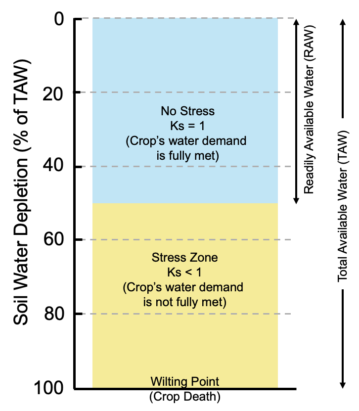
Figure 3. Illustration of how crop water demand is met under different soil moisture conditions. Crops receive full water supply when soil moisture is above the RAW threshold, but once soil water depletion exceeds RAW, water stress reduces ETc.
Rainfall, Runoff, Irrigation, Capillary Rise and Deep Percolation
The FAO-56 Method provides a more comprehensive approach to soil water balance compared to the Checkbook Method by incorporating additional components such as runoff, capillary rise, and deep percolation. While rainfall and irrigation remain the two primary sources of soil moisture, as discussed in the Checkbook Method, FAO-56 ensures that all key variables influencing soil moisture dynamics are accounted for, resulting in a more complete soil water balance. In contrast, the Checkbook Method simplifies the balance by ignoring these additional factors, which can lead to inaccurate estimations under certain field conditions.
In reality, several conditions may affect soil moisture. For instance, when light to moderate rainfall occurs, the soil soaks up water until it reaches field capacity. Any excess water beyond this threshold either drains down deep into the ground as deep percolation, where plants can’t use it, or flows over the surface as runoff into streams. If rainfall is very intense, even when the soil is not yet full, a significant portion of the rainfall may become runoff because the soil can’t absorb it quickly enough−much like how a sponge overflows if you pour water on it too fast. Additionally, in areas with a high groundwater table, water can rise upward into the root zone through small pores in the soil, a process known as capillary rise. This extra supply can increase soil moisture and sometimes reduce the need for irrigation.
By incorporating these factors, FAO-56 provides a more accurate and realistic representation of soil water dynamics, even under challenging field conditions. In contrast, the Checkbook Method, by assuming all rainfall is available water and neglecting losses from deep percolation and runoff or gains from capillary rise, fails to provide an accurate water balance under varying conditions.
Soil Water Balance Calculation
The soil water balance calculation in the FAO-56 Method integrates key hydrological processes affecting soil moisture availability in the root zone. Once all necessary data are obtained, the daily soil water depletion (Di) is computed using the equation:
Di = Di-1 – (P-RO)i – Ii – CRi + ETci + DPi (7)
where Di-1 is the root zone depletion at the end of previous day, Pi is rainfall, ROi is runoff, Ii is the net irrigation depth, CRi is capillary rise, ETci is the crop water use, and DPi is deep percolation beyond the root zone, with each term expressed in inches of water. This equation accounts for all water inputs and losses, making it more comprehensive than the Checkbook Method, which simplifies some components and does not fully incorporate soil-plant-atmosphere interactions.
Table 3 provides an example demonstrating soil water balance estimation using the FAO-56 Method. This example is referenced from Examples 35 and 38 of Allen et al.14 While the details are similar to those in Table 2, only the first 10 days are considered here for consistency with the examples in Allen et al.14
Table 3. Example of a Soil Water Balance Table Using FAO-56 Method for Irrigation Scheduling.
| Day | ETo (in/d) | Zr (in) | RAW (in) | Di start (in) | P-RO (in) | I
(in) |
Ks | Kcb | Ke | Kc | ETc (in/d) | DP (in) | Di end (in) |
| 1 | 0.18 | 11.81 | 0.92 | 0.00 | 0 | 1.57 | 1 | 0.30 | 0.91 | 1.21 | 0.22 | 0.65 | 0.22 |
| 2 | 0.20 | 12.2 | 0.95 | 0.22 | 0 | 0 | 1 | 0.31 | 0.90 | 1.21 | 0.24 | 0 | 0.46 |
| 3 | 0.15 | 12.2 | 0.95 | 0.46 | 0 | 0 | 1 | 0.32 | 0.72 | 1.04 | 0.16 | 0 | 0.62 |
| 4 | 0.17 | 12.6 | 0.98 | 0.62 | 0 | 0 | 1 | 0.33 | 0.37 | 0.70 | 0.12 | 0 | 0.74 |
| 5 | 0.19 | 12.6 | 0.98 | 0.74 | 0 | 0 | 1 | 0.34 | 0.18 | 0.52 | 0.10 | 0 | 0.84 |
| 6 | 0.11 | 12.99 | 1.01 | 0.60 | 0.24 | 0 | 1 | 0.36 | 0.64 | 1.00 | 0.11 | 0 | 0.71 |
| 7 | 0.23 | 12.99 | 1.01 | 0.71 | 0 | 0 | 1 | 0.37 | 0.45 | 0.82 | 0.19 | 0 | 0.90 |
| 8 | 0.20 | 13.39 | 1.04 | 0.90 | 0 | 0 | 1 | 0.38 | 0.17 | 0.55 | 0.11 | 0 | 1.01 |
| 9 | 0.19 | 13.39 | 1.04 | 0.01 | 0 | 1 | 1 | 0.39 | 0.08 | 0.47 | 0.09 | 0 | 0.10 |
| 10 | 0.20 | 13.78 | 1.07 | 0.10 | 0 | 0 | 1 | 0.4 | 0.81 | 1.21 | 0.24 | 0 | 0.34 |
Note. ETo and ETc represent reference and actual crop evapotranspiration, Zr is the crop root zone depth, RAW is the readily available water, P is rainfall, RO is runoff, I is the net irrigation amount, and DP is the amount of water lost through deep percolation. Ks, Kcb, Ke, and Kc correspond to water stress coefficient, basal crop coefficient, soil evaporation coefficient, and crop coefficient, respectively, while Di start and Di end represent the root zone soil moisture deficit at the start and end of day i. The highlighted Di end on Day 8 (1.01 in) indicates the soil moisture is nearing the RAW threshold of 1.04 in, prompting irrigation on Day 9.
The example assumes:
- Root zone depth (Zr): 11.81 in on Day 1 and 13.78 in on Day 10. The remaining values are interpolated.
- Soil water depletion fraction (p): 0.6.
- RAW: Calculated as:
RAW = TAW × p = (θFC – θWP) × Zr × p = (0.23-0.10) × Zr × 0.6 = 0.078 × Zr
- Root zone soil moisture depletion at the start of the day (Di start): On Day 1, Di start is set to 0 since no moisture is depleted at the beginning of the first day. From Day 2 onward, the Di start generally carries over from the previous day’s end-of-day deficit (Di-1 end), incorporating rainfall (Pi), irrigation (Ii), and deep percolation (DPi). For simplicity, capillary rise (CRi) and runoff (ROi) are assumed to be zero. Thus equation 7 is simplified as follows to compute Di start:
Di start = Di-1 end – (P-RO)i – Ii + DPi (8)
- Irrigation (I) and Rainfall (P): 1.57 in irrigation on Day 1 and 0.24 in rainfall at the beginning of Day 6.
- Water stress coefficient (Ks): Ks = 1 since soil moisture deficit doesn’t exceed RAW.
- Basal crop coefficient (Kcb): Obtained from Table 17 of Allen et al.14
- Evaporation coefficient (Ke): Values obtained from Example 35 of Allen et al.14 as it requires another set of calculations using separate soil water balance approach for topsoil layer.
- Dual crop coefficient (Kc): Obtained by summing up Kcb and Ke.
- Crop water use (ETc): Calculated using Equation 6.
- Deep Percolation (DP): If (P-RO) + I exceed RAW, then DP is their difference, otherwise 0.
- Root zone soil moisture depletion at the end of the day (Di end): Calculated as:
Di-1 = Di start + ETc (9)
Key insights from this example are outlined below:
- Early Period (Days 1–5): The initial 1.57 in irrigation keep soil moisture at adequate levels.
- Day 6: A 0.24 in rainfall event replenishes soil moisture, reducing the deficit from 0.84 in (Day 5) to 0.60 in (Day 6).
- Critical Period (Days 7–8): By Day 8, soil moisture depletion approaches the RAW threshold (1.04 in). Without irrigation, depletion would exceed the threshold.
- Irrigation Event (Day 9): A 1 in irrigation restores soil moisture to near field capacity, preventing crop stress.
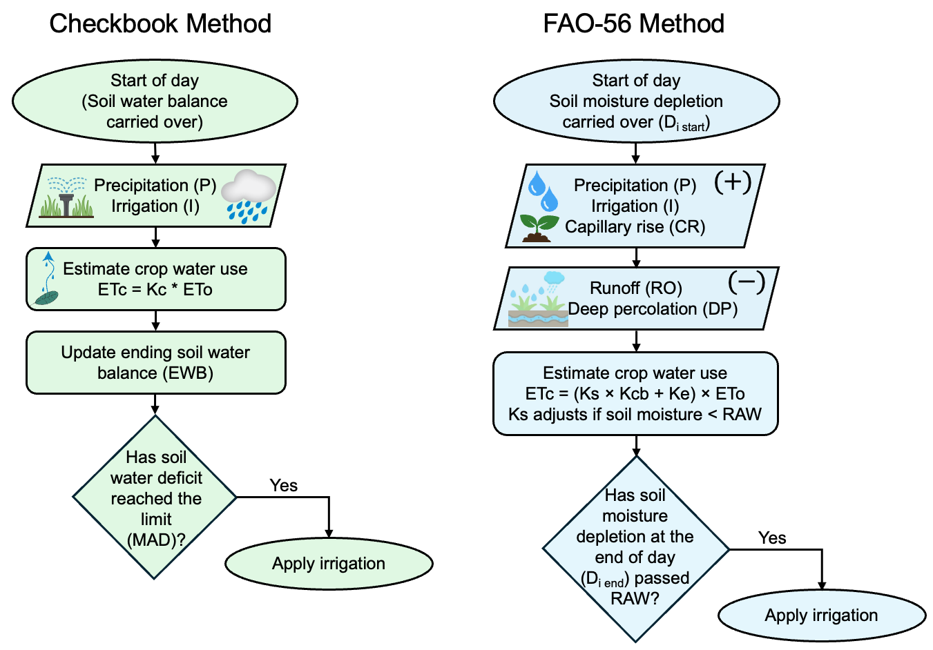
Figure 4. Flowchart summarizing the soil water balance calculations from Table 2 (Checkbook Method) and Table 3 (FAO-56 Method). This schematic provides a simplified visual comparison of the two approaches for irrigation scheduling.
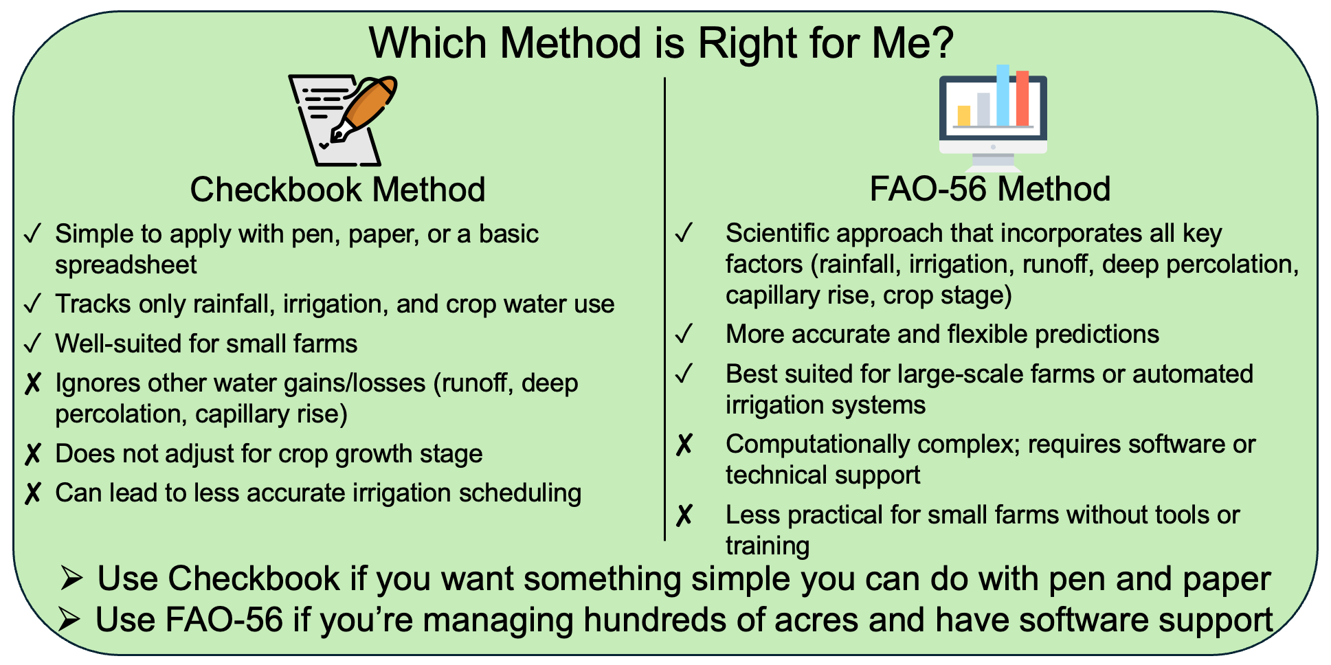
Figure 5. A side-by-side comparison of the Checkbook Method and FAO-56 Method for irrigation scheduling, showing pros and cons of each. The box concludes with an action-oriented summary: use Checkbook for simple, pen-and-paper tracking; use FAO-56 for large-scale farms with software support.
Conclusion
Irrigation scheduling plays a crucial role in optimizing crop productivity and minimizing water wastage. By ensuring that crops receive the right amount of water at the right time, effective scheduling can lead to improved yields and more sustainable water use. Two common methods for irrigation scheduling including the Checkbook Method and the FAO-56 are discussed in this article, both of which rely on soil water balance but differ in complexity and applicability.
The Checkbook Method is a simple, field-based approach that tracks major water balance components such as irrigation, rainfall, crop water use, and soil water deficit. Its simplicity makes it an attractive choice for small-scale farms, where farmers can easily apply this method. However, it uses a simplified representation of soil water balance and does not explicitly account for processes such as runoff and deep percolation, means it can sometimes overestimate available soil moisture, leading to delayed irrigation scheduling, as seen in the example calculations.
In contrast, the FAO-56 Method provides a more scientific approach to soil water balance, incorporating a broader set of factors such as runoff, deep percolation, capillary rise, and variations in soil moisture. It offers a more accurate and flexible model, particularly in accounting for the climatic and soil dynamics that affect crop water use. While this method is more complex and usually requires software to run calculations, it is ideally suited for large-scale agricultural operations or automated irrigation systems, where precision and flexibility are essential for managing water use effectively.
The example calculations illustrate how the two methods can lead to different estimates of soil moisture status and irrigation timing. These differences reflect the additional processes and assumptions incorporated in the FAO-56 framework compared with the simpler Checkbook approach.
Ultimately, the choice between the Checkbook and FAO-56 methods depends on the scale of the operation and the need for precision. While the FAO-56 Method is the preferred choice for large-scale farms, particularly those utilizing automated systems, the Checkbook Method remains a useful tool for smaller operations where simplicity and ease of implementation are more important. By understanding the strengths and limitations of each, farmers and irrigation managers can select the approach that best fits their needs, optimizing water use for sustainable and productive agriculture.
References Cited
- Allen, R. G., Pereira, L. S., Raes, D., & Smith, M. (1998). Crop evapotranspiration: Guidelines for computing crop water requirements (FAO Irrigation and Drainage Paper No. 56). Food and Agriculture Organization of the United Nations. https://www.fao.org/4/x0490e/x0490e00.htm
- Broner, I. (2005). Irrigation scheduling (Fact Sheet No. 4.708). Colorado State University Extension. https://irrigationtoolbox.com/ReferenceDocuments/Extension/Colorado/04708.pdf
- Comas, L. H., Trout, T. J., DeJonge, K. C., Zhang, H., & Gleason, S. M. (2019). Water productivity under strategic growth stage-based deficit irrigation in maize. Agricultural Water Management, 212, 433–440. https://doi.org/10.1016/j.agwat.2018.07.015
- Evans, R., Cassel, D., & Sneed, R. (2024). Soil, water and crop characteristics important to irrigation scheduling (Publication No. AG-452-01; original work published 1996). NC State Extension. https://content.ces.ncsu.edu/soil-water-and-crop-characteristics-important-to-irrigation-scheduling
- Food and Agriculture Organization of the United Nations. (n.d.). CROPWAT. Land & Water. Retrieved April 2026, from https://www.fao.org/land-water/databases-and-software/cropwat/en/
- Food and Agriculture Organization of the United Nations. (n.d.). ETo calculator. Land & Water. Retrieved February 2025, from https://www.fao.org/land-water/databases-and-software/eto-calculator/en/
- Kelly, L., Dong, Y., & Gradiz, A. (2025). Irrigation scheduling tools. Michigan State University Extension & Purdue University Extension. https://www.canr.msu.edu/irrigation/uploads/files/No%203%20-%20Irrigation%20Scheduling%20Tools%20-%20Final%20-%20June%202025.pdf
- Melvin, S. R., & Yonts, C. D. (2009). Irrigation scheduling: Checkbook method (Extension Circular EC709). University of Nebraska–Lincoln Extension. https://extensionpubs.unl.edu/publication/ec709/2009/pdf/view/ec709-2009.pdf
- National Centers for Environmental Information. (n.d.). Climate Data Online. National Oceanic and Atmospheric Administration. Retrieved August 2025, from https://www.ncdc.noaa.gov/cdo-web/search
- National Weather Service. (n.d.). Graphical forecast. National Oceanic and Atmospheric Administration. Retrieved August 2025, from https://digital.weather.gov
- Neupane, A., & Samadi, V. (2025). QuantumIrrigation: A new quantum computing Python package for irrigation demand assessment. Smart Agricultural Technology, 12, Article 101523. https://doi.org/10.1016/j.atech.2025.101523
- Nuñez, J., Haviland, D. R., Aegerter, B. J., Baldwin, R. A., Westerdahl, B. B., Trumble, J. T., & Wilson, R. G. (n.d.). UC IPM pest management guidelines: Potato (Publication 3463). University of California Agriculture and Natural Resources. Continuously revised.
- Oregon State University Small Farms Program. (n.d.). How to use Web Soil Survey to assess soil available water holding capacity. https://smallfarms.oregonstate.edu/system/files/how_to_use_web_soil_survey_to_assess_soil_available_water_holding_capacity_0.pdf
- Scherer, T., & Steele, D. (2024). Irrigation scheduling by the checkbook method (Extension Publication AE792). North Dakota State University Extension. https://www.ndsu.edu/agriculture/sites/default/files/2024-02/ae792.pdf
- Shortridge, J. (2018). Irrigation scheduling in humid climates using the checkbook method (Publication BSE-239P). Virginia Cooperative Extension. https://vtechworks.lib.vt.edu/server/api/core/bitstreams/86fc12fe-252b-4e48-96f0-d84d260e2468/content
- Thorp, K. R., DeJonge, K. C., Pokoski, T., Gulati, D., Kukal, M., Farag, F., Hashem, A., Erismann, G., Baumgartner, T., & Holzkaemper, A. (2024). pyfao56 (Version 1.3.0): FAO-56 evapotranspiration in Python. SoftwareX, 26, Article 101724. https://doi.org/10.1016/j.softx.2024.101724
- Trout, T. J., & DeJonge, K. C. (2018). Crop water use and crop coefficients of maize in the Great Plains. Journal of Irrigation and Drainage Engineering, 144(6), Article 04018009. https://doi.org/10.1061/(ASCE)IR.1943-4774.0001309
- Wright, J. (2002). Irrigation scheduling: Checkbook method (Publication FO-01322). University of Minnesota Extension Service. https://irrigationtoolbox.com/ReferenceDocuments/BasicWaterManagement/f11_irrigation_scheduling_water_budget_mn_ces.pdf